
实现输出函数
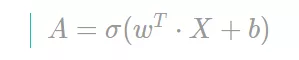
通过逻辑回归 w, b 以及输入 X,计算 Y 的预测值 A
向量化逻辑回归的输出函数
def predict(w, b, X):    '''    Arguments:    w -- 权重, 一个行向量 (num_px * num_px * 3, 1)    b -- 偏差, 一个标量    X -- 标准化后的 X 矩阵,shape 为 (num_px * num_px * 3, number of examples)
    Returns:    Y_prediction -- 一个包含了0,1,即对应 X 的预测值的向量    '''
    m = X.shape[1]    Y_prediction = np.zeros((1, m))    w = w.reshape(X.shape[0], 1)
    # 计算结果 A 为一个列向量    A = sigmoid(np.dot(w.T, X) + b)
    for i in range(A.shape[1]):        # 将列向量 A 中的可能性比率大于 0.5 作为 1, 否则为 0        Y_prediction[0, i] = 1 if A[0, i] > 0.5 else 0
    assert(Y_prediction.shape == (1, m))
    return Y_prediction
构建逻辑回归模型
调用上面已经实现的函数,构建逻辑回归模型。
def model(X_train, Y_train, X_test, Y_test, num_iterations=2000, learning_rate=0.5, print_cost=False):    '''    Arguments:    X_train -- 训练集 X 维度,shape 为 (num_px * num_px * 3, m_train)    Y_train -- 训练集 Y 维度,shape 为 (1, m_train)    X_test -- 测试集 X 维度,shape 为 (num_px * num_px * 3, m_test)    Y_test -- 测试集 Y 维度,shape 为 (1, m_test)    num_iterations -- 迭代次数/优化更新次数(超参数)    learning_rate -- 梯度下降的学习率/更新步长(超参数)    print_cost -- 是否打印损失,默认不打印
    Returns:    d -- 包含了模型详情信息的字典    '''
    # 使用 X_train 的第一维度为参数,初始化 w, b 参数    w, b = initialize_with_zeros(X_train.shape[0])
    # 梯度下降算法优化 w, b 参数    parameters, grads, costs = optimize(w, b, X_train, Y_train, num_iterations, learning_rate, print_cost)
    # 取出 w, b 参数    w = parameters["w"]    b = parameters["b"]
    # 计算训练集和测试集的预测值    Y_prediction_train = predict(w, b, X_train)    Y_prediction_test = predict(w, b, X_test)
    # 打印训练集和测试集的准确率    print("train accuracy: {} %".format(100 - np.mean(np.abs(Y_prediction_train - Y_train)) * 100))    print("test accuracy: {} %".format(100 - np.mean(np.abs(Y_prediction_test - Y_test)) * 100))

    d = {"costs": costs,         "Y_prediction_test": Y_prediction_test,          "Y_prediction_train" : Y_prediction_train,          "w" : w,          "b" : b,         "learning_rate" : learning_rate,         "num_iterations": num_iterations}
    return d
训练模型
传入参数,调用模型函数,进行训练和验证。
d = model(train_set_x, train_set_y, test_set_x, test_set_y, num_iterations = 2000, learning_rate = 0.005, print_cost = True)
Cost after iteration 0: 0.693147Cost after iteration 100: 0.584508Cost after iteration 200: 0.466949Cost after iteration 300: 0.376007Cost after iteration 400: 0.331463Cost after iteration 500: 0.303273Cost after iteration 600: 0.279880Cost after iteration 700: 0.260042Cost after iteration 800: 0.242941Cost after iteration 900: 0.228004Cost after iteration 1000: 0.214820Cost after iteration 1100: 0.203078Cost after iteration 1200: 0.192544Cost after iteration 1300: 0.183033Cost after iteration 1400: 0.174399Cost after iteration 1500: 0.166521Cost after iteration 1600: 0.159305Cost after iteration 1700: 0.152667Cost after iteration 1800: 0.146542Cost after iteration 1900: 0.140872train accuracy: 99.04306220095694 %test accuracy: 70.0 %
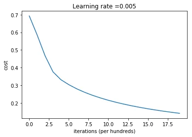
研究学习率、损失和更新次数的关系
绘制逻辑回归模型的学习曲线
costs = np.squeeze(d['costs'])plt.plot(costs)plt.ylabel('cost')plt.xlabel('iterations (per hundreds)')plt.title("Learning rate =" + str(d["learning_rate"]))plt.show()
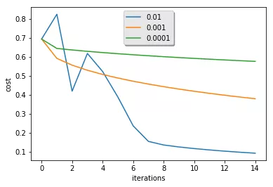
比较不同学习率下的学习曲线
learning_rates = [0.01, 0.001, 0.0001]models = {}for i in learning_rates:    print ("learning rate is: " + str(i))    models[str(i)] = model(train_set_x, train_set_y, test_set_x, test_set_y, num_iterations = 1500, learning_rate = i, print_cost = False)    print ('\n' + "-------------------------------------------------------" + '\n')
for i in learning_rates:    plt.plot(np.squeeze(models[str(i)]["costs"]), label= str(models[str(i)]["learning_rate"]))
plt.ylabel('cost')plt.xlabel('iterations')
legend = plt.legend(loc='upper center', shadow=True)frame = legend.get_frame()frame.set_facecolor('0.90')plt.show()
使用分类器
使用已经训练好的猫咪分类模型对任一图片进行分类判断。
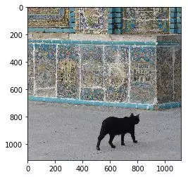
my_image = "cat_in_iran.jpg"
# 对图片预处理,使之适用于模型fname = "../input/images/" + my_image
image = np.array(plt.imread(fname))
# 查看图片plt.imshow(image)
# 使用模型进行预测,并输出结果my_image = np.array(Image.fromarray(image).resize((num_px, num_px),Image.ANTIALIAS)).reshape((1, num_px * num_px * 3)).T
my_predicted_image = predict(d["w"], d["b"], my_image)
print("y = " + str(np.squeeze(my_predicted_image)) + ", your algorithm predicts a \"" + classes[int(np.squeeze(my_predicted_image)),].decode("utf-8") +  "\" picture.")
y = 1.0, your algorithm predicts a "cat" picture.
第三章使用 TensorFlow 实现浅层神经网络进行猫咪识别
导入所需的 package
import tensorflow as tfimport numpy as npimport matplotlib.pyplot as pltfrom loadH5File import load_datafrom PIL import Image
%matplotlib inline
加载数据集 (cat / non-cat)
train_set_x, train_set_y, test_set_x, test_set_y, classes = load_data()
train_x (209, 64, 64, 3) test_x (50, 64, 64, 3)train_y (209, 1) test_y (50, 1)
其中 loadH5File 模块中定义了处理训练集和测试集 h5 文件的方法
import h5pyimport numpy as np
def load_data():    train_data = h5py.File('../input/dataset/train_catvnoncat.h5', 'r')    train_set_x = np.array(train_data['train_set_x'][:]) # train features    train_set_y = np.array(train_data['train_set_y'][:]) # train labels
    test_data = h5py.File('../input/dataset/test_catvnoncat.h5', 'r')    test_set_x = np.array(test_data['test_set_x'][:]) # test features    test_set_y = np.array(test_data['test_set_y'][:]) # test labels
    classes = np.array(test_data["list_classes"][:]) # the list of classes
    train_set_y = train_set_y.reshape(-1, 1)    test_set_y = test_set_y.reshape(-1, 1)
    print('train_x', train_set_x.shape, 'test_x', test_set_x.shape)       print('train_y', train_set_y.shape, 'test_y', test_set_y.shape)
    return train_set_x, train_set_y, test_set_x, test_set_y, classes
降维输入特征数据并归一化
# 对输入数据进行降维train_x_flatten = train_set_x.reshape(train_set_x.shape[0], -1)test_x_flatten = test_set_x.reshape(test_set_x.shape[0], -1)
# 标准化输入数据train_set_x = train_x_flatten/255test_set_x = test_x_flatten/255
print('train_x', train_set_x.shape, 'test_x', test_set_x.shape)  print('train_y', train_set_y.shape, 'test_y', test_set_y.shape)  train_x (209, 12288) test_x (50, 12288)train_y (209, 1) test_y (50, 1)
定义 batch 函数
def next_batch(X, Y, size, ind = None):    '''    Arguments:    X -- 标准化后的 X 矩阵,shape 为 (number of examples, img_size)    Y -- 一个由 0, 1 组成(其中 0 表示 non-cat, 1 表示 cat)的列向量, shape 为 (number of examples, 1)    size -- 批量处理数据的数量    ind -- 批量开始索引
    Returns:    batch_x -- 一个 X 的 batch    batch_y -- 一个 Y 的 batch    '''    if ind == None:        indexes = np.random.choice(len(X), size=size)        np.random.shuffle(indexes);      else:        indexes = np.arange(ind*size, np.where((ind+1) * size < len(X), (ind+1) * size, len(X)))
    batch_x = X[indexes]    batch_y = Y[indexes]
    return batch_x, batch_y
定义张量及计算图
# 定义训练集大小,图片维度大小num_examples = train_set_x.shape[0]img_size = train_set_x.shape[1]
# 定义学习率learning_rate = 0.002
# 初始化 x, y 占位符x = tf.placeholder(tf.float32, [None, img_size])y = tf.placeholder(tf.float32, [None, 1])
# 初始化 w, b 参数变量# W = tf.Variable(tf.zeros([img_size, 1]))# b = tf.Variable(tf.zeros([1]))W = tf.Variable(tf.random_normal([img_size, 1]))b = tf.Variable(tf.random_normal([1]))
# 前向传播计算预测值logits = tf.matmul(x, W) + by_ = tf.sigmoid(logits)
# 计算代价函数# cost = tf.reduce_mean(-1 * (y * tf.log(y_) + (1 - y) * tf.log(1 - y_))) # 计算溢出导致 cost 为 nancost = tf.reduce_mean(tf.nn.sigmoid_cross_entropy_with_logits(logits = logits, labels = y))
# 反向传播 梯度下降 优化 w, b 参数optimizer = tf.train.GradientDescentOptimizer(learning_rate=learning_rate).minimize(cost)
# 计算模型预测结果y_predict = tf.where(tf.greater(y_, np.full_like(y_, 0.5)), tf.zeros_like(y_), tf.ones_like(y_))
# 计算准确率accuracy = 100 - tf.reduce_mean(tf.cast(tf.equal(y_predict, y), tf.float32)) * 100
训练模型
# 定义其他参数batch_size = 30iter_num = 6000display_epoch = 500
# 初始化参数init = tf.global_variables_initializer()
# 启动图 (graph)sess = tf.Session()sess.run(init)
# 迭代训练,记录损失值和准确度cost_history = []train_acc = []test_acc = []
for epoch in range(iter_num):    avg_cost = 0.    avg_acuu = 0.    total_batch = int(num_examples/batch_size)
    # 循环所有 batch    for i in range(total_batch):        batch_xs, batch_ys = next_batch(train_set_x, train_set_y, batch_size, i)
        # 运行优化器,计算代价        _, c, a = sess.run([optimizer, cost, accuracy], feed_dict = {x: batch_xs, y: batch_ys})        # 累积平均成本        avg_cost += c / total_batch        avg_acuu += a / total_batch
    # 记录每个迭代成本、准确率    cost_history.append(avg_cost)    train_acc.append(avg_acuu)    test_acc.append(sess.run(accuracy, {x: test_set_x, y: test_set_y}))
    # 打印成本、准确率    if (epoch+1) % display_epoch == 0:        print('Epoch:', '%04d' % (epoch+1),              'cost=', '{:.9f}'.format(cost_history[-1]),              'train_acc=', '{:.2f}%'.format(train_acc[-1]),              'test_acc=', '{:.2f}%'.format(test_acc[-1]),             )
print('Optimization Finished!')
# 输出优化后的权重、偏差、准确率print('\nAccuracy:', '{:.2f}%'.format(test_acc[-1]), '\nWeight', sess.run(W).flatten(), '\nBias', sess.run(b).flatten())
sess.close()
Epoch: 0500 cost= 2.338835160 train_acc= 67.78% test_acc= 64.00%Epoch: 1000 cost= 1.171330139 train_acc= 84.44% test_acc= 68.00%Epoch: 1500 cost= 0.600112927 train_acc= 91.11% test_acc= 70.00%Epoch: 2000 cost= 0.311668488 train_acc= 96.11% test_acc= 66.00%Epoch: 2500 cost= 0.145401367 train_acc= 97.78% test_acc= 68.00%Epoch: 3000 cost= 0.078871274 train_acc= 98.89% test_acc= 66.00%Epoch: 3500 cost= 0.050911599 train_acc= 99.44% test_acc= 66.00%Epoch: 4000 cost= 0.037607569 train_acc= 99.44% test_acc= 64.00%Epoch: 4500 cost= 0.029192524 train_acc= 99.44% test_acc= 64.00%Epoch: 5000 cost= 0.023540985 train_acc= 99.44% test_acc= 64.00%Epoch: 5500 cost= 0.019640291 train_acc= 100.00% test_acc= 64.00%Epoch: 6000 cost= 0.016851171 train_acc= 100.00% test_acc= 64.00%Optimization Finished!
Accuracy: 64.00% Weight [-1.3992907   0.5485633  -0.13500667 ...  0.9261457   1.6744033 -0.507459  ] Bias [-0.33652216]
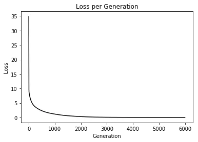
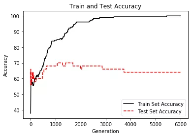
绘制模型评估曲线
# 绘制损失和准确度曲线plt.plot(cost_history, 'k-')plt.title('Loss per Generation')plt.xlabel('Generation')plt.ylabel('Loss')plt.show()
# 绘制训练集、测试集准确率曲线plt.plot(train_acc, 'k-', label='Train Set Accuracy')plt.plot(test_acc, 'r--', label='Test Set Accuracy')plt.title('Train and Test Accuracy')plt.xlabel('Generation')plt.ylabel('Accuracy')plt.legend(loc='lower right')plt.show()
第四章使用 Keras 实现深度神经网络进行猫咪识别
导入所需的 package
from keras.models import Sequentialfrom keras.layers import Densefrom keras.optimizers import SGDimport numpy as npimport matplotlib.pyplot as pltfrom loadH5File import load_datafrom PIL import Image
%matplotlib inlineUsing TensorFlow backend.
加载数据集 (cat / non-cat)
train_set_x, train_set_y, test_set_x, test_set_y, classes = load_data()
train_x (209, 64, 64, 3) test_x (50, 64, 64, 3)train_y (209, 1) test_y (50, 1)
降维输入特征数据并归一化
# 偏平化输入特征train_x_flatten = train_set_x.reshape(train_set_x.shape[0], -1)test_x_flatten = test_set_x.reshape(test_set_x.shape[0], -1)
# 标准化输入数据train_set_x = train_x_flatten/255test_set_x = test_x_flatten/255
print('train_x', train_set_x.shape, 'test_x', test_set_x.shape)  print('train_y', train_set_y.shape, 'test_y', test_set_y.shape) train_x (209, 12288) test_x (50, 12288)train_y (209, 1) test_y (50, 1)
搭建深度神经网络
# 定义训练集大小,图片维度大小num_examples = train_set_x.shape[0]img_size = train_set_x.shape[1]
model = Sequential()model.add(Dense(256, activation="relu", input_shape=(img_size,)))model.add(Dense(128, activation="relu"))model.add(Dense(64, activation="relu"))model.add(Dense(32, activation="relu"))model.add(Dense(1, activation="sigmoid"))
查看神经网络
model.summary()_________________________________________________________________Layer (type) Output Shape Param # =================================================================dense_1 (Dense) (None, 256) 3145984 _________________________________________________________________dense_2 (Dense) (None, 128) 32896 _________________________________________________________________dense_3 (Dense) (None, 64) 8256 _________________________________________________________________dense_4 (Dense) (None, 32) 2080 _________________________________________________________________dense_5 (Dense) (None, 1) 33 =================================================================Total params: 3,189,249Trainable params: 3,189,249Non-trainable params: 0_________________________________________________________________
编译模型
model.compile(optimizer=SGD(), loss="binary_crossentropy", metrics=['accuracy'])
开始训练
history = model.fit(train_set_x, train_set_y, epochs=20, validation_data=(test_set_x, test_set_y), verbose=1)
Train on 209 samples, validate on 50 samplesEpoch 1/20209/209 [==============================] - 1s 4ms/step - loss: 0.6918 - acc: 0.5789 - val_loss: 0.8544 - val_acc: 0.3400Epoch 2/20209/209 [==============================] - 0s 645us/step - loss: 0.6483 - acc: 0.6459 - val_loss: 0.8409 - val_acc: 0.3400Epoch 3/20209/209 [==============================] - 0s 647us/step - loss: 0.6270 - acc: 0.6507 - val_loss: 0.9070 - val_acc: 0.3400Epoch 4/20209/209 [==============================] - 0s 721us/step - loss: 0.6206 - acc: 0.6507 - val_loss: 0.9309 - val_acc: 0.3400Epoch 5/20209/209 [==============================] - 0s 645us/step - loss: 0.6367 - acc: 0.6651 - val_loss: 0.9284 - val_acc: 0.3400Epoch 6/20209/209 [==============================] - 0s 609us/step - loss: 0.6073 - acc: 0.6555 - val_loss: 0.9694 - val_acc: 0.3400Epoch 7/20209/209 [==============================] - 0s 646us/step - loss: 0.6028 - acc: 0.6555 - val_loss: 0.8310 - val_acc: 0.3400Epoch 8/20209/209 [==============================] - 0s 633us/step - loss: 0.5790 - acc: 0.6842 - val_loss: 0.7948 - val_acc: 0.3400Epoch 9/20209/209 [==============================] - 0s 605us/step - loss: 0.5653 - acc: 0.7081 - val_loss: 0.7247 - val_acc: 0.3600Epoch 10/20209/209 [==============================] - 0s 694us/step - loss: 0.5807 - acc: 0.6842 - val_loss: 0.9499 - val_acc: 0.3400Epoch 11/20209/209 [==============================] - 0s 704us/step - loss: 0.5729 - acc: 0.7129 - val_loss: 0.6200 - val_acc: 0.8000Epoch 12/20209/209 [==============================] - 0s 668us/step - loss: 0.5491 - acc: 0.7703 - val_loss: 0.6280 - val_acc: 0.7400Epoch 13/20209/209 [==============================] - 0s 678us/step - loss: 0.5316 - acc: 0.7321 - val_loss: 0.7044 - val_acc: 0.5800Epoch 14/20209/209 [==============================] - 0s 671us/step - loss: 0.4940 - acc: 0.8086 - val_loss: 0.8441 - val_acc: 0.3600Epoch 15/20209/209 [==============================] - 0s 747us/step - loss: 0.5148 - acc: 0.7416 - val_loss: 0.7896 - val_acc: 0.3400Epoch 16/20209/209 [==============================] - 0s 730us/step - loss: 0.4917 - acc: 0.7990 - val_loss: 0.6306 - val_acc: 0.7200Epoch 17/20209/209 [==============================] - 0s 723us/step - loss: 0.5081 - acc: 0.8134 - val_loss: 0.6794 - val_acc: 0.5600Epoch 18/20209/209 [==============================] - 0s 683us/step - loss: 0.5363 - acc: 0.7081 - val_loss: 1.0372 - val_acc: 0.3400Epoch 19/20209/209 [==============================] - 0s 725us/step - loss: 0.4456 - acc: 0.8038 - val_loss: 0.5148 - val_acc: 0.7800Epoch 20/20209/209 [==============================] - 0s 719us/step - loss: 0.4556 - acc: 0.8278 - val_loss: 0.7439 - val_acc: 0.4800
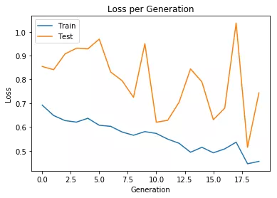
绘制训练曲线
# 绘制训练 & 验证的损失值plt.plot(history.history['loss'])plt.plot(history.history['val_loss'])plt.title('Loss per Generation')plt.ylabel('Loss')plt.xlabel('Generation')plt.legend(['Train', 'Test'], loc='upper left')plt.show()
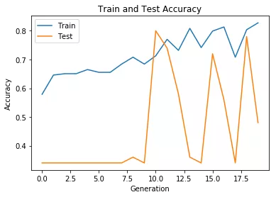
# 绘制训练 & 验证的准确率值plt.plot(history.history['acc'])plt.plot(history.history['val_acc'])plt.title('Train and Test Accuracy')plt.ylabel('Accuracy')plt.xlabel('Generation')plt.legend(['Train', 'Test'], loc='upper left')plt.show()
总结
在实战中,我们可以很明显的观察到,准确率在达到一个阈值后就无法再提升了,我们通常把这种情况称为过拟合,这是拟合高方差的结果。为此可以采取一系列措施解决,如 L2 正则、随机失活、数据扩增、提前结束迭代训练等等,这些是在调整神经网络模型中常用的方法,这里不再详述。
相信大家通过阅读,已经大概了解神经网络的基础,以及了解如何实现一个神经网络,Tensorflow、Keras 的使用和体验。在机器学习框架的选择上,个人建议可以考虑 Keras 这个更高阶的框架,十分适合初学者。
只有不断编程实战才能加强神经网络建模和参数优化的能力,希望感兴趣的同学看过这篇文章可以有所得,谢谢大家。
作者介绍:
江伯(企业代号名),目前负责贝壳找房经纪人作业和横向技术相关工作。
本文转载自公众号贝壳产品技术(ID:gh_9afeb423f390)。
原文链接:
https://mp.weixin.qq.com/s/THlhGRKC5tfF2XxRNcIoZg
更多内容推荐
深度学习 keras 像搭积木般构建神经网络模型
用Keras搭建神经网络的步骤,7大部分就可以轻松构建模型。介绍了主要的API调用以及注意事项。
2021-03-31
11|VAE 系列:如何压缩图像给 GPU 腾腾地方
这一讲,我们将一起了解VAE的基本原理,之后我们训练自己的Stable Diffusion模型时,也会用上VAE这个模块。
2023-08-09
怎样让深度学习模型更泛用?
不变风险最小化是一种激动人心的新型学习范式,可帮助预测模型的泛化水平超越训练数据的局限。
如何使用 TensorFlow 构建机器学习模型
在这篇文章中,我将逐步讲解如何使用TensorFlow创建一个简单的机器学习模型。
主动学习:如何用更少的数据做更多的事情?
我使用了主动学习,仅利用了 23% 的实际训练数据集(ATIS 意向分类数据集)来实现与 100% 数据集训练相同的结果。
如何使用 TFX 中的 NSL 框架实现图的正则化?
NSL是 TensorFlow 中的一个框架,可用于训练具有结构化信号的神经网络。
作为一名机器学习工程师,需要了解哪些神经网络的可解释性?
想要打开算法“黑盒”,了解神经网络的可解释性十分重要。
如何使用半监督学习为结构化数据训练出更好的深度学习模型
本文将使用半监督学习来提高深度神经模型在低数据环境下应用于结构化数据时的性能。
为什么我的模型表现这么差?
阅读本文,你将学到如何识别这些现象的必要的知识,并获得如何克服这些现象的工具和补救措施,最终提高你的模型性能,这是每一个机器学习工程师的真正目标。
颠覆者扩散模型:直观去理解加噪与去噪
扩散模型的工作原理是怎样的呢?算法优化目标是什么?与GAN相比有哪些异同?这一讲我们便从这些基础问题出发,开始我们的扩散模型学习之旅。
2023-07-28
深度广度模型在用户购房意愿量化的应用
在部分场景如点击率预估中,输入的特征一般为大规模稀疏矩阵,如何对输入进行有效表达就成了深度学习在点击率预估中应用的关键所在。
10|CLIP:让 AI 绘画模型乖乖听你的话
只有真正理解了CLIP,你才能知道为什么prompt可以控制AI绘画生成的内容。
2023-08-07
机器学习笔记(二):线性回归
本文为华为云系列文章之一。
深度学习正在被滥用
在某些情况下,神经网络之类模型的表现可能会胜过更简单的模型,但很多情况下事情并不是这样的。
为什么机器学习模型会失败?
本文用一个真实的例子解决了模型不能得到足够好的结果的问题。
22|YouTubeDNN:召回算法的后起之秀(下)
上节课我们讲了关于YouTubeDNN的召回模型,接下来,我们来看看如何用代码来实现它。
2023-06-05
12|实战项目(二):动手训练一个你自己的扩散模型
今天,我们将通过实战的形式,一起训练一个标准扩散模型,并微调一个Stable Diffusion模型,帮你进一步加深对知识的理解。
2023-08-11
08|巧用神经网络:如何用 UNet 预测噪声
今天我就来为你解读UNet的核心知识。搞懂了这些,在你的日常工作中,便可以根据实际需求对预测噪声的模型做各种魔改了,也会为我们之后训练扩散模型的实战课打好基础。
2023-08-02
如何解决机器学习算法执行表现不佳的问题
如果你的机器学习算法没有达到预期的效果,那下一步该怎么办?
机器学习笔记(一):基本概念
本文是作者在机器学习方面的学习笔记。
推荐阅读
16|ChatGPT:是什么让 LLM 走向舞台中央?
2023-09-15
竞赛:糖尿病遗传风险检测挑战赛(科大讯飞)
2022-08-02
BP 神经网络(算法整体思路及原理 + 手写公式推导)
2022-07-06
27|模型工程(三):低成本领域模型方案,小团队怎么做大模型?
2023-10-20
如期而至 - 用户购买时间预测(下)
2021-12-10
26|模型工程(二):算力受限,如何为“无米之炊”?
2023-10-18
PGL 图学习之图神经网络 ERNIESage、UniMP 进阶模型 [系列八]
2022-11-26
电子书

大厂实战PPT下载
换一换 
汪晟杰 | 腾讯云 开发者产品中心/产品总监
姚立 | 字节跳动 架构前端平台架构 团队负责人
张柳青 | 百度 资深研发工程师


评论